Homework 2: NBody

A. Goals

The goal of the NBody assignment is to familiarize you with arrays, iteration, graphics, and Java command-line arguments. The specific goals are to:

Learn about a scientific computing application
Learn to build up complex results using a sequence of simple statements
Reinforce understanding of animations
Use nested loops
Use arrays
Use Java command-line arguments

At the end of this assignment, you will have produced a visual simulation of the gravitational interactions among particles in two dimensions.

B. Background

In 1687, in his famous Principia, Sir Isaac Newton formulated the principles governing the motion of two particles under the influence of their mutual gravitational attraction. However, Newton was unable to solve the problem for three particles. Indeed, in general, systems of three or more particles can only be solved numerically.

Your challenge in this assignment is to write a program to simulate the motion of numParticles particles in the plane that are mutually affected by gravitational forces, and animate the results. Such methods are widely used in astronomy, semiconductors, and fluid dynamics to study complex physical systems. Scientists also apply the same techniques to other pairwise interactions including Coulombic, Biot-Savart, and van der Waals.

We provide all the formulas you need in the assignment. Don't worry if you don't fully understand them – this is neither a physics nor a math course. Instead, focus on the computer science task: building up a complicated result through a series of simple statements.

C. Your Program

We are going to use Newton's universal law of gravitation and Java to simulate the manner in which celestial bodies interact. Since we are most familiar with the solar system, the primary objective is to create a simulation showing the planets (Mercury through Mars) orbiting around the Sun. Here's what your end result will look like.

Each body in the simulation has three characteristics that define its movement: its position, its velocity (the speed and direction of movement), and its acceleration (the rate and direction of change of the particle’s velocity).

At each timeStep in your simulation, you will draw all particles in their proper location. Then, for each pair of particles A and B, you will find the gravitational force that B exerts on A based on their respective masses and the distance between them using Newton’s Law of Gravitation. Since there is a force acting on A, Newton’s Second Law of Motion predicts that A will accelerate (i.e., its velocity will change). You will then compute A's new velocity. After finding the new velocities of all of the particles, you will compute their new positions, which will be displayed on the simulation.

D. Getting Started

Create a Java class called NBody with an empty main() function. Give your file a header comment.

Download and compile PennDraw.java into the same folder as NBody.java.

Download nbody_data.zip and decompress it into the same folder as NBody.java.

E. Advice

Compile, run, and debug frequently; make one small change at a time, ensuring that your program works as you expect it to after each change.
Be certain to debug and test your program as you go. Even if you have not yet gotten to steps with graphical output, you can test your program easily by adding in temporary System.out.println() statements. For instance, if you read in a variable, print its value to check that the value of the variable is the value you expect. If you do a computation, print out the result and check it. Once you're certain the variable is correct, you can remove these temporary System.out.println() statements.
Keep your code organised by using indentation and avoiding too many blank lines.
Comment frequently and use good variable names.
Examine debugging errors in the console for clues as to what went wrong.

Refresher: Using Command-Line Arguments

If you'd like a refresher on how command-line arguments work, please review this example. Otherwise, move onto part A in this section.

A Java program can take arguments when it is executed from the command-line at the Interactions pane. These arguments are passed to the main() function as a String array called args; thus, the first command-line argument is args[0], the second is args[1], and so on.

public class CommandLineArguments {
    public static void main(String[] args) {
        System.out.println(args.length);
        System.out.println(args[0]);
        System.out.println(Double.parseDouble(args[1]));
        System.out.println(Integer.parseInt(args[2]));
    }
}

Compile this program (you may cut and paste it into DrJava if you like) and run it by clicking Run on the toolbar. What happens?

Open the Interactions pane and enter these commands at the prompt:

java CommandLineArguments benedict 2.0 3
java CommandLineArguments
java CommandLineArguments benedict
java CommandLineArguments benedict 2.0 3 arvind
java CommandLineArguments benedict arvind 3
java CommandLineArguments benedict 2 3
java CommandLineArguments benedict 2 3.0

Make sure you understand each line of code, and why you get the output and runtime errors that you do for each set of command-line arguments.

A. NBody's Command-Line Arguments

Your NBody program will take three command-line arguments:

first, a double representing how long your simulation should run
second, a double representing how much time should pass for each timeStep
third, a string for the filename where the universe information is stored

Declare three variables simulationTime, timeStep, and filename and assign them to their respective command line arguments.

B. Checkpoint

Compile NBody and run it with the command line arguments 15778000.0, 25000.0, and solarSystem.txt. Your program should not crash. If it does, use System.out.println() to isolate and rectify the bug. Any debugging code that you add should be commented out when you submit.

A. Input File Format

Your NBody program will be pulling data from a file in order to setup its simulation. This data will include a list of all the particles, their masses, initial positions, etc. By storing the simulation's specifications in a separate file, we can write a simulator that can load and simulate a variety of scenarios.

This separate data file will be a text file of the following format.

5        numParticles 
2.50e+11 radius 
5.97400e+24  1.49600e+11  0.00000e+00  0.00000e+00  2.98000e+04    earth.gif
6.41900e+23  2.27900e+11  0.00000e+00  0.00000e+00  2.41000e+04     mars.gif
3.30200e+23  5.79000e+10  0.00000e+00  0.00000e+00  4.79000e+04  mercury.gif
1.98900e+30  0.00000e+00  0.00000e+00  0.00000e+00  0.00000e+00      sun.gif
4.86900e+24  1.08200e+11  0.00000e+00  0.00000e+00  3.50000e+04    venus.gif
m[]          px[]         py[]         vx[]         vy[]             img[]

In this file,

numParticles is the number of particles in the simulation
radius is the radius of the universe; your simulation will assume that all particles will have x- and y-coordinates between -radius and radius
There will be numParticles rows remaining in the file, each containing six values:
- m[] is the mass of the particle in kilograms (m)
- px[] and py[] are the initial x- and y-coordinates of the particle in metres (p_x, p_y)
- vx[] and vy[] are the initial x- and y-components of the particle velocity in metres per second ( v_x, v_y)
- img[] is the filename of the image file used to represent the particle in the simulation

B. Setting Up `inStream`

The booksite's standard library provides the file In.java to support reading from a file. Study StudentsFileProcessor.java, which is contained in the nbody_data.zip you downloaded in Part 0. It is an example of reading from a file. Compile StudentsFileProcessor.java, and run it from the DrJava Interactions Pane with the argument students.txt:

java StudentsFileProcessor students.txt

In your NBody class, declare and initialise a variable, inStream, as below:

 In inStream = new In(filename); // creates a variable inStream to read from the file

C. Reading Values From The File

Now that inStream is initialised, you can read from it using the following function calls. These functions behave identically to those in StdIn.

boolean b = inStream.isEmpty();     // boolean value that is true if there are no more values, false otherwise
int     i = inStream.readInt();     // reads in an int from inStream
double  d = inStream.readDouble();  // reads in a double from inStream
boolean b = inStream.readBoolean(); // reads in a boolean from inStream
String  s = inStream.readString();  // reads in a string from inStream
String  s = inStream.readLine();    // reads in an entire line from inStream
String  s = inStream.readAll();     // reads in the entire file from inStream

inStream will start reading from the beginning of the file. Each time a function like inStream.readDouble() is called, inStream interprets the next number as a double (an error will occur if it cannot be parsed to a double). The next time a read function is called, inStream moves to the next item in the file.

For example, say that a file, sample.txt, is as follows:

4 5

The code snippet

In inStream = new In("sample.txt");
int x = inStream.readInt();
double y = inStream.readDouble();

will set x to 4 and y to 5.0.

In your NBody program, declare an integer variable numParticles and a double variable radius. Using the above functions, assign to numParticles and radius the first and second values in the file, respectively.

D. Reading Arrays from the File

Declare double arrays m, px, py, vx, and vy, and String array img, and initialise them to length numParticles. Use the inStream functions and a loop to read the values in the numParticles lines in the file.

E. Checkpoint

Copy the code below and paste it at the end of your main() function.

System.out.printf("%d\n", numParticles);
System.out.printf("%.2e\n", radius);
for (int i = 0; i < numParticles; i++) {
    System.out.printf("%12.5e %12.5e %12.5e %12.5e %12.5e %12s\n", m[i], px[i], py[i], vx[i], vy[i], img[i]);
}

Compile your program and run it with the same arguments: 15778000.0, 25000.0, and solarSystem.txt. Note that by pressing ↑ you can recall commands previously typed into the Interactions pane. The output from the Interactions pane should exactly match the text in the file solarSystem.txt. If your program crashes or if the output is different, use System.out.println()statements to isolate and rectify the bug. Any debugging code that you add should be commented out (but not deleted) when you submit.

A. The Background

The scale of the simulation window should be from -radius to radius in both the x, and y direction. Use PennDraw's setXscale and setYscale to do this.

Use PennDraw's PennDraw.picture() to draw the image starfield.jpg in the center window.

B. The Particles

Using a loop, draw each particle in its respective position. Note that the i^th particle's x position is stored as px[i]. Find the y position and image filename similarly.

C. Checkpoint

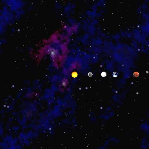
Compile and run your code using the command-line arguments 15778000.0, 25000.0, and solarSystem.txt. This should show all five particles in a line on a starfield background image like so:

NBody still

A. The Time Loop

You will need to wrap your simulation in a loop, where each iteration of the loop represents one step in time. In each step, the particle's positions must be updated and their images redrawn.

Begin by writing this loop. You will need to declare a variable representing how much time has elapsed. This should increase by timeStep each step, and should be used to determine when the elapsed time has exceeded the simulationTime -- at that point, the simulation should halt. The structure of your loop should enforce these requirements.

Once you have your loop, add a call to PennDraw.enableAnimation(30) before your loop begins. You may adjust the frame rate by changing the number if you'd like (higher will make the animation faster, lower will make it slower). Also, add a call to PennDraw.advance() within your time loop.

B. Update Particle Positions

Inside the time loop but before redrawing the particles, update each particle's positions. If a particle's initial position is (p_x, p_y), its updated position should be at (p_x + Δt v_x, p_y + Δt v_y). Δt represents the change in time of the motion of our particles.

C. Checkpoint

Compile and run your code using the command-line arguments 15778000.0, 25000.0, and solarSystem.txt (same as before). The planets should now be moving straight up and off the screen, and the sun should be staying put at the center of the screen.

If the animation flickers or smears, check that you are drawing the background only once per iteration of the time loop.

D. Update Particle Velocity

Outer loop – For every particle A, you must compute the forces exerted on it by every other particle B. This outer loop will use the net force on particle A, F_x and F_y, to calculate the acceleration of A and update its velocity. See above image for the formulas on how to calculate F_x and F_y. We suggest that you declare variables for each calculation you see in the image. (Your variable names should respect the camel case naming conventions of Java variables rather than the the convential symbols used in physics.)

Inner loop – The net force exerted on particle A should be the sum of the forces exerted on it by each other particle B. Define variables to hold the x - and y-components of the force exerted by particle B on A. Hint: Each iteration of the inner loop should increase the net force F_x and F_y on particle A by the force exerted by particle B on A in the x - and y-directions. When the inner loop finishes for particle A, the values of F_x and F_y should be the net force components for particle A that will be used to calculate its acceleration. (Your variable names should respect the camel case naming conventions of Java variables rather than the the convential symbols used in physics.)

force diagram

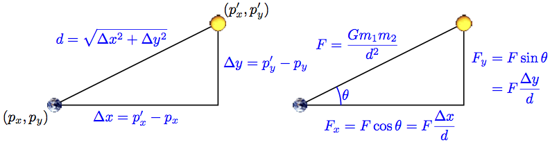
Δx and Δy – Be careful computing Δx and Δy. These are the distances in the x- and y-directions from the first planet to the second one, and can be negative. You should not take the absolute value of the differences between their x- and y-positions.

Gravity – Define a variable G for the gravitational constant so the formulas will be easier to read. Initialize it to the value 6.67e-11. When calculating the force between particle A and B, use the following order of operations to avoid NaN values: ((G * m_A) / (d * d)) * m_B

Acceleration – By Newton's Second Law, for each particle, the resultant acceleration components of that particle are a_x = F_x / m and a_y = F_y / m. Compute the x- and y-components of the particle's acceleration.

Velocity – Using the acceleration you just computed, update the velocity (v_x, v_y) to (v_x + Δt a_x, v_y + Δt a_y). This gives you the new direction and speed of each particle.

Order of computation – It is imperative to update the velocity of every particle before updating any positions. Even though your program computes these velocities one after the other, you have to maintain the illusion that all planets are moving at the same time. For instance, if you update the Earth's position before computing Mars' velocity, then you will end up computing Mars' velocity based on Earth's future position, rather than its current position.

E. Common Problems

Anti-Gravity – If you flip the order of your particles when you compute Δx and Δy, your particles will repel rather than retract each other. For the solarSystem.txt example, you might end up with something that looks like this:

Planets jump to the upper-left corner – Check your loop for computing the pairwise forces between particles. Are you computing the force exerted by a particle on itself (e.g. Earth's gravitational pull on itself)? If you are, do the computation by hand to see exactly what it would give you. That should help you understand why this is a bad idea, and why the planets jump the way they do. (Video is slowed for illustration.)

Planets go around the sun, then zoom off the lower left corner – You are not summing up the pairwise forces correctly. Run your program with a small value of simulationTime (e.g. 51000) so it runs for only two or three time steps. Print out the value of every variable before and after you change its value (or right after you first initialize it). Include enough information in the print statement so you can tell which variable you are printing out. Make sure to print all loop variables as well so you can tell from the output exactly when each print statement occured. Run the program, and examine the output. Ask yourself each time a variable changes whether its starting and new values make sense. (You don't need to work out the exact values of the variables to figure out if they make sense in this case.) Once you've found the problem, you may want to move the declarations of some variables farther inside your loops to the first point you need them. Declaring variables as late as possible is one strategy to avoid the type of bug you are encountering. (Video is slowed for illustration.)

Planets are flickering – You are either not calling PennDraw.advance() at all, or calling it after drawing each particle instead of after drawing all particles. This means each planet appears to move as soon as you draw it, instead of all the planets appearing to move in sync.

Planets are flickering, and only one shows at a time – You are redrawing the background before drawing each planet, instead of redrawing it once per timeStep. As a result, you keep covering up each planet as soon as you draw it.

Planets "smear" accross the screen – You are drawing the background once at the beginning of the programming instead of once each time step. PennDraw does not erase the window automatically. In this program, we're never erasing it at all. Instead, we keep covering the old planet positions up with the starfield image, which happens to be exactly the same size as the window. If you don't keep redrawing the background before drawing the planets at their new positions, the old planets are still there, causing the smearing effect.

F. Checkpoint

Compile and run your program. The particles should now orbit the Sun, and at the end of the simulation, your program should print the final state of the system.

The following are the values you should obtain for the final state of the system with various values of simulationTime and timeStep. When testing, you should start with a single time step, making sure that it is working completely. Then try a small number of time steps, again making certain that it is working completely, before going on to a full year. It is much easier to diagnose problems for smaller time frames.

java NBody 25000.0 25000.0 solarSystem.txt (one step)

5
2.50e+11
5.97400e+24  1.49596e+11  7.45000e+08 -1.48201e+02  2.98000e+04    earth.gif
6.41900e+23  2.27898e+11  6.02500e+08 -6.38597e+01  2.41000e+04     mars.gif
3.30200e+23  5.78753e+10  1.19750e+09 -9.89331e+02  4.79000e+04  mercury.gif
1.98900e+30  3.30867e+01  0.00000e+00  1.32347e-03  0.00000e+00      sun.gif
4.86900e+24  1.08193e+11  8.75000e+08 -2.83294e+02  3.50000e+04    venus.gif

java NBody 50000.0 25000.0 solarSystem.txt (two steps)

5
2.50e+11
5.97400e+24  1.49589e+11  1.48998e+09 -2.96404e+02  2.97993e+04    earth.gif
6.41900e+23  2.27895e+11  1.20500e+09 -1.27720e+02  2.40998e+04     mars.gif
3.30200e+23  5.78258e+10  2.39449e+09 -1.97887e+03  4.78795e+04  mercury.gif
1.98900e+30  9.92618e+01  2.81978e-01  2.64700e-03  1.12791e-05      sun.gif
4.86900e+24  1.08179e+11  1.74994e+09 -5.66597e+02  3.49977e+04    venus.gif

java NBody 75000.0 25000.0 solarSystem.txt (three steps)

5
2.50e+11
5.97400e+24  1.49578e+11  2.23493e+09 -4.44605e+02  2.97978e+04    earth.gif
6.41900e+23  2.27890e+11  1.80748e+09 -1.91579e+02  2.40995e+04     mars.gif
3.30200e+23  5.77516e+10  3.59045e+09 -2.96820e+03  4.78386e+04  mercury.gif
1.98900e+30  1.98523e+02  1.12801e+00  3.97047e-03  3.38411e-05      sun.gif
4.86900e+24  1.08158e+11  2.62477e+09 -8.49891e+02  3.49931e+04    venus.gif

java NBody 31557600.0 25000.0 solarSystem.txt (one year)

5
2.50e+11
5.97400e+24  1.49594e+11 -1.65312e+09  3.29492e+02  2.97978e+04    earth.gif
6.41900e+23 -2.21530e+11 -4.92633e+10  5.18050e+03 -2.36404e+04     mars.gif
3.30200e+23  3.47713e+10  4.57516e+10 -3.82694e+04  2.94146e+04  mercury.gif
1.98900e+30  5.94260e+05  6.23570e+06 -5.85686e-02  1.62847e-01      sun.gif
4.86900e+24 -7.37309e+10 -7.93909e+10  2.54335e+04 -2.39734e+04    venus.gif

You should also test your program against some of the other universes that we provided. Ensure that your program does not misbehave when given more or fewer than five particles.

G. Music

This task is not for credit; it is just for fun. (Depending on the individual configuration of your personal computer, this may not work correctly.) Add the following line somewhere before your time loop:

StdAudio.play("2001.mid");

Run your program again, and let us know in the readme whether you have sound. The music is the fanfare to Also sprach Zarathustra by Richard Strauss; it was popularised as the key musical motif in Stanley Kubrick’s 1968 film 2001: A Space Odyssey.

A. Extra credit

Submit a .zip file called extra.zip containing an alternate universe (in our input format) along with the necessary image files. If its behavior is sufficiently interesting, we'll award extra credit. Your submission must be in a zip file, even if there are no images, so that our grading scripts can handle it correctly.

B. Technical details on the simulation

This simulation method is called the leapfrog finite difference approximation scheme; it is based on a numeric integration of Newton’s equations, and is the basis for most astrophysical simulations of gravitational systems.

The leapfrog method is more stable for integrating Hamiltonian systems than conventional numerical methods like Euler’s method or Runge-Kutta. The leapfrog method is symplectic, which means it preserves properties specific to Hamiltonian systems (conservation of linear and angular momentum, time-reversibility, and conservation of energy of the discrete Hamiltonian). In contrast, ordinary numerical methods become dissipative and exhibit qualitatively different long-term behavior. For example, the Earth would slowly spiral into (or away from) the Sun. For these reasons, symplectic methods are extremely popular for N-body calculations in practice.

Here’s a more complete explanation of how you should interpret the variables. The classic Euler method that updates the position of the particles uses the velocity at time t instead of using the updated velocity at time t + Δt. A better idea is to use the velocity at the midpoint, t + Δt / 2. The leapfrog method does this in a clever way. It maintains the position and velocity one-half time step out of phase: at the beginning of an iteration, (p_x, p_y) represents the position at time t whilst (v_x, v_y) represents the velocity at time t - Δt / 2. Interpreting the position and velocity in this way, the updated position (p_x + Δt v_x, p_y + Δt v_y) uses the velocity at time t + Δt / 2. Almost magically, the only special care needed to deal with the half time-steps is to initialize the system’s velocity at time t = Δt / 2 (instead of t = 0.0), and you can assume that we have already done this for you in solarSystem.txt. Note also that the acceleration is computed at time t so that when we update the velocity, we are using the acceleration at the midpoint of the interval under consideration.

A. Readme

Complete readme_nbody.txt in the same way that you have done for previous assignments.

B. Submission

Submit NBody.java and readme_nbody.txt on the course website. If you completed the extra credit, also submit extra.zip.

Prior to submission remove any print statements used for debugging.

Homework 2: NBody

A. Goals

B. Background

C. Your Program

D. Getting Started

E. Advice

Refresher: Using Command-Line Arguments

A. NBody's Command-Line Arguments

B. Checkpoint

A. Input File Format

B. Setting Up inStream

C. Reading Values From The File

D. Reading Arrays from the File

E. Checkpoint

A. The Background

B. The Particles

C. Checkpoint

A. The Time Loop

B. Update Particle Positions

C. Checkpoint

D. Update Particle Velocity

E. Common Problems

F. Checkpoint

G. Music

A. Extra credit

B. Technical details on the simulation

A. Readme

B. Submission

B. Setting Up `inStream`