Homework 2: N-Body Simulation

Goals

Learn about a scientific computing application.
Learn about reading input using the StdIn library and printing formatted output using the StdOut library.
Learn about plotting graphics using the StdDraw library.
Learn about using the command line to redirect standard input to read from a file.
Learn to build up complex results using a sequence of simple statements
Use nested loops
Use arrays.

Submission

Submit NBody.java and a completed readme_nbody.txt file using the submission link in the sidebar.

Background

In 1687 Sir Isaac Newton formulated the principles governing the the motion of two particles under the influence of their mutual gravitational attraction in his famous Principia. However, Newton was unable to solve the problem for three particles. Indeed, in general, systems of three or more particles can only be solved numerically. Your challenge is to write a program to simulate the motion of N particles in the plane, mutually affected by gravitational forces, and animate the results. Such methods are widely used in cosmology, semiconductors, and fluid dynamics to study complex physical systems. Scientists also apply the same techniques to other pairwise interactions including Coulombic, Biot-Savart, and van der Waals.

We provide all the formulas you need in the assignment. Don't worry if you don't fully understand them: this is neither a physics nor a math course. Instead, focus on the computer science task: building up a complicated result through a series of simple statements.

Your program. Write a program NBody.java that:

Reads two double command-line arguments T and Δt.
Reads in the universe from standard input using StdIn.
Simulates the universe, starting at time t = 0.0, and continuing as long as t < T, using the procedure describe below.
Animates the results to standard drawing using StdDraw.
Prints the state of the universe at the end of the simulation (in the same format as the input file) to standard output using StdOut.

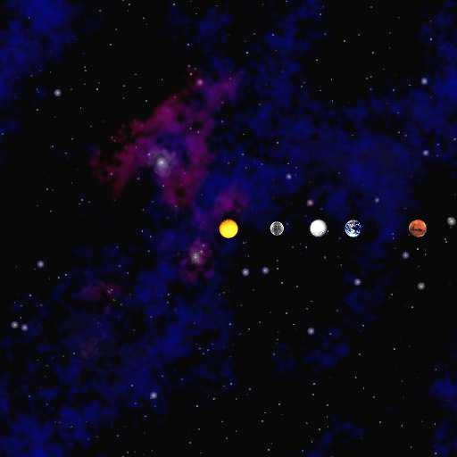
Maintain several parallel arrays to store the data. To make the computer simulation, write a loop that repeatedly updates the position and velocity of the particles.

The end result of your program should like like the following:

Part I: Reading Input

Download nbody_data.zip and unzip it into the same directory as NBody.java.
Read Section 1.5. Review Students.java included in the zip file for help with standard input and parallel arrays. Compile and execute this program to make sure your system is configured properly. You can use the included file students.txt as input, but you will need to run this from the terminal/command prompt since input redirection doesn't work in DrJava:
```
% java Students < students.txt
```
If you have trouble compiling Students.java, check the Common Problems section below. The booksite's standard library may not be correctly configured on your computer.
Input format. The input format is a text file that contains the information for a particular universe.
1. The first value is an integer N that represents the number of particles.
2. The second value is a real number R that represents the radius of the universe: assume all particles will have x- and y-coordinates that remain between -R and R.
3. The remaining N rows, each contain 6 values. The first two are the x- and y-coordinates of the initial position (px[] and py[]); the second two are the x- and y-components of the initial velocity (vx[] and vy[]); the fifth is the mass (m[]); the last is a String that is the name of an image file used to display the particle (image[]). As an example, planets.txt contains data for our solar system (in SI units).
Read in the data file planets.txt from standard input as described above. Copy the code below into your program to print it out in the same format. Right now, you are printing the information to aid in debugging; later, you will use this code to print out the state of the universe at the end of the simulation.
```
StdOut.printf("%d\n", N);
StdOut.printf("%.2e\n", R);
for (int i = 0; i < N; i++) {
    StdOut.printf("%11.4e %11.4e %11.4e %11.4e %11.4e %12s\n",
                   px[i], py[i], vx[i], vy[i], m[i], image[i]);
}
```
You should compile your program in Dr. Java, but you will need to run your program from the terminal/command prompt because it is impossible to redirect standard input from a file within Dr. Java. Open the Terminal (Mac) or Command Prompt (Windows), and use the cd command to change directories (folders) to the one where you program is located. Then type, for example:
% java NBody 15778000.0 25000.0 < planets.txt
Your program should print out the contents of planets.txt just as they appear above. You can ignore the two command-line arguments for now, which control the time simulation, and focus on the reading planets.txt.
Do not even think of continuing until you have tested and debugged this part.

Part II: Draw the Planets

Review DeluxeBouncingBall.java included in the zip file for help with StdDraw, including how to use StdDraw.show() for smooth animation. There are many methods in StdDraw, but for this assignment, you won't need more than the ones that are used in DeluxeBouncingBall.java. The required image and sound files are also in the zip.
Set the scale of the window to show the entire universe using StdDraw.setXscale(-R, R) and StdDraw.setYscale(-R, R). Since you only need to set the scale once, you should put these near the top of your program before any loops or other StdDraw code.
Plot the background starfield.jpg image included in the zip. Note that StdDraw.picture(x, y, file) centers the picture on (x, y). starfield.jpg should be centered at (0, 0). Test that it works. Now, write a loop to plot the N bodies. If all goes correctly, you should see the four stationary planets and the sun.

Part III: Making the Planets Move

Background: The motion of particles is governed by a set of equations known as Newton's laws of motion and gravitation. (At the scale of the galaxy, we can treat planets as particles.) The equations contain two basic parts: velocity, which is the speed and direction that a particle is moving, and acceleration which are changes to speed and acceleration. Particles always move in a straight line at a constant speed unless some outside force (e.g. friction, gravity, or a push) creates an acceleration that changes the speed or direction. In our simulations, the only force will be gravity. First, however, we suggest implementing a universe without gravity and testing to make sure this works.

Although we think of time as advancing continuously and of objects as moving continuously, computers are not good at simulating constant change. Instead, we settle for letting time jump forward in discrete time steps of Δt, measured in seconds, called the time quantum. Particles will simply jump from the old position to the new position at each time step. By settings Δt very small, we can get a very accurate simulation, but will need to do an enormous number of computations. Setting it very large will make the simulation very fast, but not very accurate. The scheme for doing this simulation, which we describe in detail below, is called the leapfrog finite difference approximation scheme. It numerically integrate Newton's equations (don't worry if that statement is meaningless to you), and is the basis for most astrophysical simulations of gravitational systems.

The Time Loop
- Use Double.parseDouble() to read the two command-line arguments from args[0] and args[1] into variables T and dt. T is the time at which your simulation should end (the end of the universe, if you will), and dt is the amount of time that should pass in each step of your simulation.
  The latter is normally written "Δt" in formulas, but variable names are limited to Roman alphabet.
- Write a loop around the code that draws your planets to control the time component of your simulation. Because T and dt are command-line arguments, rather than part of the input file, you can simulate the same universe at different speed and for different lengths of time.
- If you haven't already added a call to StdDraw.show(20) in your code, add one after you've drawn all your planets, but inside the loop. The argument "20" controls the speed of the animation; you can increase it to speed up the animation or decrease it to slow the animation down. Without it your animation will flicker, and if it is too short you animation may not run smoothly.
- Make sure your program compiles. There should be no change yet when you run it.
Calculate new position for every planet
- Inside the loop, before you redraw the planets, update the position (p_x, p_y) to (p_x + Δt v_x, p_y + Δt v_y). Remember that the positions and velocities of your planets are stored in the px, py, vx, and vy arrays.
- Compile and run your program. For the planets.txt input, the sun should stay put in the center of the window, and the four planets should move straight up and off the screen. This is because their initial velocities specified in planets.txt all point straight up and we have not yet incorporated accelearation.
- If your animation flickers or smears, check the Common Problems section below.
Calculate new velocity for every planet
- Gravitational Forces (Background): To update the particle velocities at each time step, you need to to compute the gravitational forces. Since the force depends on the relative positions of particles, it changes constantly and must be inside your time loop. On the other hand, you need it to update the velocities and therefore the positions, so it must come at the beginning of the time loop. The acceleration of a single particle, say the planet Earth, is simply the sum of forces exerted by all other planets on it (the principle of superposition). For each planet, you will need a loop over all other planets to sum up the force they exert on it. You will need to do this for all planets.
- Gravitational Forces (Scaffolding Code): For now, assume the force that any planet exerts on any other planet is 0. (You will update this in the following steps.) Write code to compute the total force on each planet by summing up the pairwise forces as described above. The result will of course be zero, but will let you focus on the pairwise forces in the next step. Make sure your code compiles at the end of this and every step.
- Pairwise Gravitational Forces: The formula for the pairwise force F that one particle exerts on another is known as Newton's law of universal graviation. It is the gravitational constant 6.67 × 10^-11 Nm²/kg² times the product of the two particles' masses, divided by the distance between them. The following figure illustrates the formula, using the Earth and the sun as representative particles:
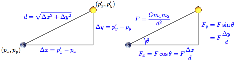
- x- and y- Force Components: Since the velocity is broken down into x- and y- components, the force needs to be too. Write code to compute the pairwise forces F_x and F_y using the formulas from the figure. Don't try and write this as one big formula; instead, write in in several small steps just as it is on the figure. Don't worry if you don't fully understand the formulas. That's the computer's job.
- Style and Readability Improvement: Define a variable G for the gravitational constant at the top of your program, so the formulas will be easier to read. Initialize it to the value 6.67e-11. This is Java-speak for 6.67× 10^-11.
- Δx and Δy: Be careful computing Δx and Δy. These are the distances in the x- and y- directions from the first planet to the second one, and can be negative. You should not take the absolute value of the differences between their x- and y- positions.
- Acceleration: Compute the acceleration on each particle using the formulas a_x = F_x / m and a_y = F_y / m where m is the mass of the particle, and F_x and F_y are the sum of all pairwise forces exerted on the particle.
  This is Newton's second law of motion.
- Velocity: Using the acceleration you just computed, update the velocity (v_x, v_y) to (v_x + Δt a_x, v_y + Δt a_y). This gives you the direction and speed each particle should move at the current time, taking into account the gravitational pull of every other particle.
- Order of computation: Remember that you must update the velocity of every particle before you can update any positions. Even though your program computes these velocities one after the other, you have to maintain the illusion that all planets are moving at the same time. For instance, if you update the Earth's position before computing Mars's velocity, then you will end up computing Mars's velocity based on Earth's future position, rather than its current position.
- Testing: Compile and run your program. The planets should now orbit the sun.

After completing this section, review the requirements in Your Program at the top of this page, and make sure you are fulfilling the requirements exactly. Continue testing with other input files.

Sound

For an optional finishing touch, play the theme to 2001: A Space Odyssey using StdAudio and the file 2001.mid. It's a one-liner using the method StdAudio.play(). On some computers, this adds a delay when the program starts up. For this reason, we recommended adding sound only when everything else works. It's entirely optional and not worth any points.

Common Problems

Standard Libraries Missing For this assignment, you need to use the booksite's standard libraries. If you ran the introcs installer, these should be set up for you, and everything should "just work." If not, you may need to download StdIn.java, Draw.java, StdDraw.java, and StdAudio.java into the same folder as your NBody.java.
My planets fly off the top right corner of the screen. You have probably flipped the order of particles when computing Δx and Δy. As a result, the signs on all your distances are all reversed, and gravity is repelling planets from each other instead of attracting them. (Video is slowed for illustration.)
My planets all disappear or jump to the top left corner as soon as I start running the program. Check your loop for computing the pairwise forces between particles. Are you computing the force exerted by a particle on itself (e.g. Earth's gravitational pull on itself)? If you are, do the computation by hand to see exactly what it would give you. That should help you understand why this is a bad idea, and why the planets jump the way they do. (Video is slowed for illustration.)
My planets go around the sun, then zoom off the lower left corner. You are not summing up the pairwise forces correctly. Run your program with a small value of T (e.g. 51000) so it runs for only two or three time steps. Print out the value of every variable before and after you change its value (or right after you first initialize it). Include enough information in the print statement so you can tell which variable you are printing out. Make sure to print all loop variables as well so you can tell from the output exactly when each print statement occured. Run the program, and examine the output. Ask yourself each time a variable changes whether its starting and new values make sense. (You don't need to work out the exact values of the variables to figure out if they make sense in this case.) Once you've found the problem, you may want to move the declarations of some variables farther inside your loops to the first point you need them. Declaraing variables as late as possible is one strategy to avoid the type of bug you are encountering. (Video is slowed for illustration.)
My planets are flickering. You are either not calling StdDraw.show() at all, or calling it after drawing each particle instead of after drawing all particles. This means each planet appears to move as soon as you draw it, instead of all the planets appearing to move in sync.
My planets are flickering, and I only see one of them at a time. You are redrawing the background before drawing each planet, instead of redrawing it once per timestep. As a result, you keep covering up each planet as soon as you draw it.
My planets "smear" accross the screen. You are drawing the background once at the beginning of the programming instead of once each time step. StdDraw does not erase the window automatically. In this program, we're never erasing it at all. Instead, we keep covering the old planet positions up with the starfield image, which happens to be exactly the same size as the window. If you don't keep redrawing the background before drawing the planets at their new positions, the old planets are still there, causing the smearing effect.

More Precise Testing

Below are the outputs your program should print after running on the planets.txt for various lengths of time. Make sure you are printing your output at the very end of the program before comparing to these. The exact numbers you get may be slightly different than the ones below if you do your computations in a slightly different order than our solution. This is fine, and is caused by rounding errors that affect the results differently depending on the precise order of statements. The biggest errors will appear to be in the sun's position. Don't worry; all the values are printed in scientific notation. The planets' positions all end in e+10 or e+11, meaning you should multiple the numbers by 10¹⁰ or 10¹¹. The exponents on the sun's position are on the scale of 10⁵. An error in the leading digit of the sun's position is therefore miniscule compared to the planet positions. Another way to think about this is that the window is 512 × 512 pixels, representing coordinates ranging from -2.5 × 10¹¹ to 2.5 × 10¹¹. Even if the leading digit of the sun's position is off by one, the error is on the order of 10000, which is far less that one pixel in the window!

Here are our results for a few sample inputs.

% java NBody 0.0 25000.0 < planets.txt           // zero steps
5
2.50e+11
 1.4960e+11  0.0000e+00  0.0000e+00  2.9800e+04  5.9740e+24    earth.gif
 2.2790e+11  0.0000e+00  0.0000e+00  2.4100e+04  6.4190e+23     mars.gif
 5.7900e+10  0.0000e+00  0.0000e+00  4.7900e+04  3.3020e+23  mercury.gif
 0.0000e+00  0.0000e+00  0.0000e+00  0.0000e+00  1.9890e+30      sun.gif
 1.0820e+11  0.0000e+00  0.0000e+00  3.5000e+04  4.8690e+24    venus.gif

% java NBody 25000.0 25000.0 < planets.txt       // one step
5
2.50e+11
 1.4960e+11  7.4500e+08 -1.4820e+02  2.9800e+04  5.9740e+24    earth.gif
 2.2790e+11  6.0250e+08 -6.3860e+01  2.4100e+04  6.4190e+23     mars.gif
 5.7875e+10  1.1975e+09 -9.8933e+02  4.7900e+04  3.3020e+23  mercury.gif
 3.3087e+01  0.0000e+00  1.3235e-03  0.0000e+00  1.9890e+30      sun.gif
 1.0819e+11  8.7500e+08 -2.8329e+02  3.5000e+04  4.8690e+24    venus.gif

% java NBody 50000.0 25000.0 < planets.txt       // two steps
5
2.50e+11
 1.4959e+11  1.4900e+09 -2.9640e+02  2.9799e+04  5.9740e+24    earth.gif
 2.2790e+11  1.2050e+09 -1.2772e+02  2.4100e+04  6.4190e+23     mars.gif
 5.7826e+10  2.3945e+09 -1.9789e+03  4.7880e+04  3.3020e+23  mercury.gif
 9.9262e+01  2.8198e-01  2.6470e-03  1.1279e-05  1.9890e+30      sun.gif
 1.0818e+11  1.7499e+09 -5.6660e+02  3.4998e+04  4.8690e+24    venus.gif

% java NBody 60000.0 25000.0 < planets.txt       // three steps
5
2.50e+11
 1.4958e+11  2.2349e+09 -4.4460e+02  2.9798e+04  5.9740e+24    earth.gif
 2.2789e+11  1.8075e+09 -1.9158e+02  2.4099e+04  6.4190e+23     mars.gif
 5.7752e+10  3.5905e+09 -2.9682e+03  4.7839e+04  3.3020e+23  mercury.gif
 1.9852e+02  1.1280e+00  3.9705e-03  3.3841e-05  1.9890e+30      sun.gif
 1.0816e+11  2.6248e+09 -8.4989e+02  3.4993e+04  4.8690e+24    venus.gif


% java NBody 31557600.0 25000.0 < planets.txt    // one year
5
2.50e+11
 1.4959e+11 -1.6531e+09  3.2949e+02  2.9798e+04  5.9740e+24    earth.gif
-2.2153e+11 -4.9263e+10  5.1805e+03 -2.3640e+04  6.4190e+23     mars.gif
 3.4771e+10  4.5752e+10 -3.8269e+04  2.9415e+04  3.3020e+23  mercury.gif
 5.9426e+05  6.2357e+06 -5.8569e-02  1.6285e-01  1.9890e+30      sun.gif
-7.3731e+10 -7.9391e+10  2.5433e+04 -2.3973e+04  4.8690e+24    venus.gif

Extra Credit

Submit a zip file containing an alternate universe (in our input format) along with the necessary image files. If its behavior is sufficiently interesting, we'll award extra credit. Your submission must be in a zip file, even if there are no images, so that our grading scripts can handle it correctly.

Challenge for the Bored

There are limitless opportunities for additional excitement and discovery here. Try adding other features, such as supporting elastic or inelastic collisions. Or, make the simulation three-dimensional by doing calculations for x-, y-, and z-coordinates, then using the z-coordinate to vary the sizes of the planets. Add a rocket ship that launches from one planet and has to land on another. Allow the rocket ship to exert force with the consumption of fuel.

Enrichment

What is the music in 2001.mid? It's the fanfare to Also sprach Zarathustra by Richard Strauss. It was popularized as the key musical motif in Stanley Kubrick's 1968 film 2001: A Space Odyssey.
I'm a physicist. Why should I use the leapfrog method instead of the formula I derived in high school? In other words, why does the position update formula use the velocity at the updated time step rather than the previous one? Why not use the 1/2 a t^2 formula? The leapfrog method is more stable for integrating Hamiltonian systems than conventional numerical methods like Euler's method or Runge-Kutta. The leapfrog method is symplectic, which means it preserves properties specific to Hamiltonian systems (conservation of linear and angular momentum, time-reversibility, and conservation of energy of the discrete Hamiltonian). In contrast, ordinary numerical methods become dissipative and exhibit qualitatively different long-term behavior. For example, the earth would slowly spiral into (or away from) the sun. For these reasons, symplectic methods are extremely popular for N-body calculations in practice. You asked!
Here's a more complete explanation of how you should interpret the variables. The classic Euler method updates the position uses the velocity at time t instead of using the updated velocity at time t + Δt. A better idea is to use the velocity at the midpoint t + Δt / 2. The leapfrog method does this in a clever way. It maintains the position and velocity one-half time step out of phase: At the beginning of an iteration, (p_x, p_y) represents the position at time t and (v_x, v_y) represents the velocity at time t - Δt / 2. Interpreting the position and velocity in this way, the updated position (p_x + Δt v_x, p_y + Δt v_y). uses the velocity at time t + Δt / 2. Almost magically, the only special care needed to deal with the half time-steps is to initialize the system's velocity at time t = -Δt / 2 (instead of t = 0.0), and you can assume that we have already done this for you. Note also that the acceleration is computed at time t so that when we update the velocity, we are using the acceleration at the midpoint of the interval under consideration.
Here are some interesting two-body systems, perhaps relevant to the extra credit. Here is beautiful 21-body system in a figure-8 - reproducing this one will definitely earn you extra credit.
Here is a website that generates music using an N-body simulator!
N-body simulations play a crucial role in our understanding of the universe. Astrophysicists use it to study stellar dynamics at the galactic center, stellar dynamics in a globular cluster, colliding galaxies, and the formation of the structure of the Universe. The strongest evidence we have for the belief that there is a black hole in the center of the Milky Way comes from very accurate N-body simulations. Many of the problems that astrophysicists want to solve have millions or billions of particles. More sophisticated computational techniques are needed.
The same methods are also widely used in molecular dynamics, except that the heavenly bodies are replaced by atoms, gravity is replaced by some other force, and the leapfrog method is called Verlet's method. With van der Waals forces, the interaction energy may decay as 1/R^6 instead of an inverse square law. Occasionally, 3-way interactions must be taken into account, e.g., to account for the covalent bonds in diamond crystals.

CIS 110 Spring 2013 - Introduction to Computer Programming